David Ziganto
David Ziganto is a senior data scientist and corporate trainer at Metis in Chicago, IL. This post was originally shared on his site at https://dziganto.github.io/, but we enjoyed it so much we wanted to share it with everyone.
Introduction
In my last post, Sparse Matrices For Efficient Machine Learning, I showcased methods and a workflow for converting an in-memory data matrix with lots of zero values into a sparse matrix with Scipy. This did two things:
- compressed the in-memory footprint of the data matrix
- sped up many machine learning routines
I ended that post with a challenge: if the original data matrix won’t fit into memory in the first place, can you think of a way to convert it to a sparse matrix anyway?
To solve this problem we need to think bigger. We need to step away from in-memory techniques and instead take our first step into out-of-core, or on-disk, methods.
In this vein, allow me to introduce Hierarchical Data Format version 5 (HDF5), an extremely powerful tool rife with capabilities. As best summarized in the book Python and HDF5
[mkd_blockquote text=”“HDF5 is just about perfect if you make minimal use of relational features and have a need for very high performance, partial I/O, hierarchical organization, and arbitrary metadata”.” title_tag=”h4″ width=””]
Let’s pause for a second. Before I go any further allow me to set the stage. I could have taken a very different approach to this post. I could have started with the very basics of HDF5 talking about things like datasets, groups, and attributes. That naturally would have led to a discussion about hierarchical organization, on-the-fly data compression, and partial I/O. I could have then gone on to describe h5py, a Pythonic interface to HDF5. However, I decided my primary goal in this post is to whet your appetite and, more importantly, to provide code and applications that you can use immediately. To that end I decided to leverage a data object from another powerful tool called PyTables that sits atop HDF5. The reason I did this is simple. Pandas and the table object from PyTables work together seamlessly. This allows me to store pandas dataframes in the HDF5 file format. It also provides a simple way to use numerous on-the-fly compressors as well as varying levels of compression. The point is that pandas and the table format in PyTables make it easy to work with the dataframes we’re all familiar with but in a way that can leverage the powerful capabilities of HDF5.
On that note, I will focus predominately on the compression capabilities available in HDF5. That is not to say the myriad other capabilities are any less important. Quite to the contrary. Instead I want this post to be an extension of the last in which we discussed data compression, albeit the in-memory type.
So let’s move beyond in-memory methods and begin our out-of-core journey with on-disk data compression, starting with a brief description of the dataset with which we’ll work.
Dataset: Dota 2
 Dota 2 is a popular computer game published by Valve Corporation. Two teams consisting of five players are forged from among 113 heroes, each with unique strengths and weaknesses. Players and teams gain experience and items during the course of the game, which ends when one team destroys the “Ancient”, a structure in the opposing team’s base.
I chose the Dota2 Games Results Data Set because:
- it is real-world data.
- it comes from the UCI repo which is a great resource.
- it is about gaming and who doesn’t like that?
The dataset captures information for all games played in a space of 2 hours on the 13th of August, 2016. Specifically, the dataset consists of a target variable and 116 features. The target variable is coded -1 and 1 for dire victory and radiant victory, respectively where “dire” and “radiant” are names of each team. Three features provide game information and the remaining 113 features indicate if a particular hero was played for a given game. The dataset is reasonably sparse as only 10 of 113 possible heroes are chosen in a given game. Furthermore, the data was pre-split into training and test sets and zipped into a single file.
Fundamentally, this is a classification problem where one team wins and one team loses. No ties are allowed. The goal here is not to showcase classification algorithms. Rather, the goal is to introduce HDF5 and to show you how to use pandas to read/write files from/to the HDF5 format with compression.
Caveats: while HDF5 has partial I/O capabilities baked in and partial I/O is extremely important from a machine learning perspective, this post will not delve into details. That will come in a future post. However, you should at least be aware that HDF5 natively has that ability. Additionally, while I am including the bulk of the code from my notebook, all the gory details can be found here for those interested.
Setup
import pandas as pd
import numpy as np
import h5py
Get Data
The zip file from UCI includes two files: one train and one test. Pandas has zip/unzip functionality but can only handle zip files with a single dataset. Since this particular zip file had a training dataset and a test dataset zipped into the same file, I had to preprocess the zip file to prep it for pandas. Here is my code:
# get zip data from UCI
import requests, zipfile, StringIO
r = requests.get("https://archive.ics.uci.edu/ml/machine-learning-databases/00367/dota2Dataset.zip")
z = zipfile.ZipFile(StringIO.StringIO(r.content))
Now we can read the datasets into pandas like so:
# get train data
X_train = pd.read_csv(z.open('dota2Train.csv'), header=None)

# get test data
X_test = pd.read_csv(z.open('dota2Test.csv'), header=None)
DF to HDF5 Conversion
Let’s convert these dataframes into HDF5 using three compressors set to max compression. You should update filepath to save your data appropriately.
compressors = ['blosc', 'bzip2', 'zlib']
for compressor in compressors:
    X_train.to_hdf('filepath_' + str(compressor) + '.h5',
                   'table', mode='w', append=True, complevel=9, complib=compressor)
    X_test.to_hdf('filepath_' + str(compressor) + '.h5',
                   'table', mode='w', append=True, complevel=9, complib=compressor)
In the next section I will show the impact of these compression procedures. Before I do, however, now is a good time to discuss the compression/decompression process. First, let’s begin with an in-memory object. In our case we’ll assume it is a pandas dataframe. When we write the data to disk in the HDF5 format, what happens? The dataframe gets converted to a PyTables table object. That object is then compressed using whichever compression filter and compression level is selected. This is an on-the-fly compression procedure because there is a compression function that acts on the in-memory object before writing to storage. Keep in mind the reverse case in which we start with a compressed data object. Once initiated, an on-the-fly decompressor ingests the stored data, decompresses it, and pushes it into memory. So we get compression on-disk but that object gets decompressed going back into memory. The point is that you cannot use this method to store a compressed data object in-memory. It is merely meant to compress data on-disk. Remember that.
File Sizes
Here I will calculate the original raw file size and the file size of each compressed file using blosc, bzip2, and zlib filters.
# get original file size (in MB)
import os
original_size = []
datasets = ['Train', 'Test']
for dataset in datasets:
    original_size.append( round(os.path.getsize("filepath" + str(dataset) + ".csv")/1e6, 2) )
original_data_size = zip(datasets, original_size)

# get compressed file sizes (in MB)
compressed_size = []
for compressor in compressors:
    for dataset in datasets:
        compressed_size.append( round(os.path.getsize("filepath" + dataset + "_" + str(compressor) + ".h5")/1e6, 2) )
compressed_data_size = zip(sorted(['blosc', 'bzip2', 'zlib']*2), ['train', 'test']*3, compressed_size)

# get sizes of compressed objects
train_compressed_size = [compressed_data_size[i][2] for i in range(0,len(compressed_data_size),2)]
test_compressed_size = [compressed_data_size[i][2] for i in range(1,len(compressed_data_size),2)]
# append original size values
train_compressed_size.append(original_data_size[0][1])  ## append original train data size
test_compressed_size.append(original_data_size[1][1])  ## append original test size
# reorder list
myorder=[3,0,1,2]
train_compressed_size = [ train_compressed_size[i] for i in myorder]
test_compressed_size = [ test_compressed_size[i] for i in myorder]
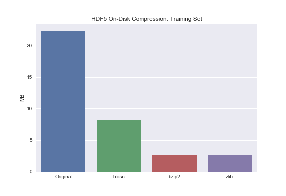
Barplot of Training Set for comparison:
sns.barplot(['Original', 'blosc', 'bzip2', 'zlib'], train_compressed_size)
plt.ylabel('MB')
plt.title('HDF5 On-Disk Compression: Training Set');
 Barplot of Test Set for comparison:
sns.barplot(['Original', 'blosc', 'bzip2', 'zlib'], test_compressed_size)
plt.ylabel('MB')
plt.title('HDF5 On-Disk Compression: Test Set');
 You may notice that bzip2 and zlib compress the data to roughly the same extent. Blosc, on the other hand, does significantly compress the data but not to the same extent as bzip2 or zlib. Why is that? Turns out there exists this tradeoff between total compression and read/write times. Zlib and bzip2 are great if your main concern is on-disk storage – not read/write though. If your primary concern is read/write times but you still want to leverage on-disk compression, use blosc.
Compressors
We just saw three compressors that drastically reduced the size of our dataset. You are probably wondering how they work. Since each one could be a post unto itself, I will simply leave it to the reader to follow the links below to learn more.
blosc
High-level Blosc
Technical Blosc
HDF5 Blosc
Blosc Benchmarks on Genotype Data
bzip2
bzip2 Overview
bzip2 Wikipedia
zlib
Back to our dataset…
spy()
That’s right, I’m bringing Matplotlib’s spy() back.
I use spy() to get a sense of the data’s sparsity. Since the data is long and skinny (92,650 x 117), I transpose it so we can get a better view. Also, I am only capturing the first 1000 rows. Why? Because the dimensions of the dataset are highly skewed which causes the image to get compressed. In other words, the visualization gets crunched so bad that we cannot discern anything useful otherwise.
fig = plt.figure(figsize=(15,8))
plt.spy(X_train.transpose().ix[:, :1000]);
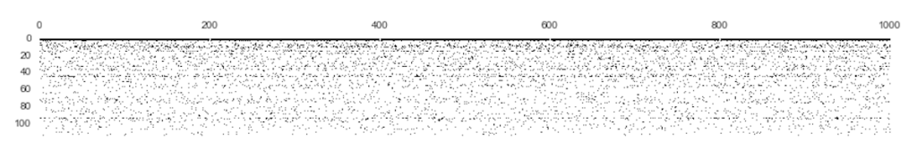 You can see the data is very sparse in all but the first three features. The next logical step is to convert it to a sparse matrix using Scipy’s CSR algorithm.
In-Memory Compression
# Preprocessing
## separate target var from dataset
y_train = X_train.pop(0)
y_test = X_test.pop(0)

## change indicator values from -1, 0, 1 to 0, 1
X_train = X_train.abs()
X_test = X_test.abs()
Let’s use CSR to compress this in-memory dataset and compare data footprints.
from scipy.sparse import csr_matrix
X_train_sparse = csr_matrix(X_train)

dense_size = np.array(X_train).nbytes/1e6
sparse_size = (X_train_sparse.data.nbytes + X_train_sparse.indptr.nbytes + X_train_sparse.indices.nbytes)/1e6

sns.barplot(['DENSE', 'SPARSE'], [dense_size, sparse_size])
plt.ylabel('MB')
plt.title('In-Memory Compression');
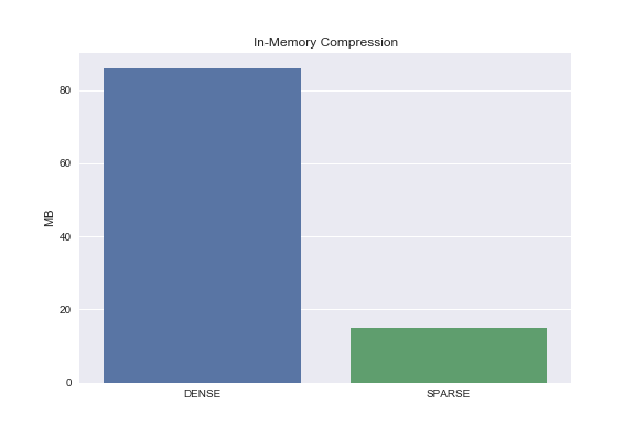 Yay, compression!
Takeaway: we now have the capability to compress data both in-memory and on-disk; this capability will serve us well in the future as we tackle online learning.
Machine Learning
In my previous post I indicated that sparse matrix implementations can dramatically speed up machine learning algorithms. If you read that post you may have noticed that I created dummy data to test my hypothesis. Now that we have Dota2 data, real-world data, this is the perfect opportunity to see if my logic holds up.
BernoulliNB
from sklearn.naive_bayes import BernoulliNB
nb = BernoulliNB(alpha=1.0, binarize=None, fit_prior=True, class_prior=None)
%timeit nb.fit(X_train, y_train)
%timeit nb.fit(X_train_sparse, y_train)
PassiveAggressiveClassifier
from sklearn.linear_model import PassiveAggressiveClassifier
pac = PassiveAggressiveClassifier(C=1.0, fit_intercept=True, n_iter=5, shuffle=True, verbose=0, loss='hinge',
                                  n_jobs=-11, random_state=12, warm_start=False, class_weight=None)
%timeit pac.fit(X_train, y_train)
%timeit pac.fit(X_train_sparse, y_train)
Perceptron
from sklearn.linear_model import Perceptron
percept = Perceptron(penalty='l2', alpha=0.001, fit_intercept=True, n_iter=20, shuffle=True, verbose=0, eta0=1.0, n_jobs=-1,
                     random_state=37, class_weight=None, warm_start=False)
%timeit percept.fit(X_train, y_train)
%timeit percept.fit(X_train_sparse, y_train)
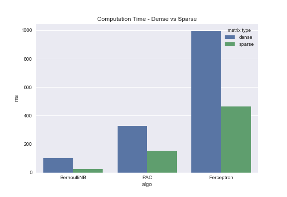 Quite a contrast. Again, this is a real dataset that was pulled from the UCI Machine Learning Repo. This isn’t some contrived example. Test it for yourself.
Summary
What are the big takeaways here?
- If you walk away with nothing else, be aware that HDF5 is a powerful tool that provides on-the-fly compression/decompression and partial I/O capabilities.
- For those less skilled in working with zip files, hopefully you learned how to take a zip file composed of multiple datasets and read them straight into pandas without having to download and/or unzip anything first.
- For those new to HDF5, hopefully you learned how to convert in-memory dataframes to HDF5 using compression.
- Sparse matrices make many machine learning algorithms faster.
Let me leave you with this: we may not know how to take a sparse matrix that won’t fit into RAM and crunch it down just yet, but taking a step into what is known as out-of-core computation puts us a tad closer.