John Readey, The HDF Group
Introduction
If you’ve spent much time working with public repositories of HDF5 data, you’ll often see data organized as a large collection of files where the files are organized by time, geographic location or both. For example, the NCEP3 climate data repository (https://disc.gsfc.nasa.gov/datasets/GSSTF_NCEP_3/summary) published by NASA, consists of 7855 files covering data from July 1, 1987 to December 31, 2009. Each file provides data for one day in this period with a filename of the pattern: GSSTF_NCEP.3.YYYY.MM.DD.he5.
Each of these 7855 files have the same layout in terms of groups, links, dataset shape, and type with just the dataset data differing between the files. For example:
$ h5ls -r GSSTF_NCEP.3.1987.07.01.he5
/ Group
/HDFEOS Group
/HDFEOS/ADDITIONAL Group
/HDFEOS/ADDITIONAL/FILE_ATTRIBUTES Group
/HDFEOS/GRIDS Group
/HDFEOS/GRIDS/NCEP Group
/HDFEOS/GRIDS/NCEP/Data\ Fields Group
/HDFEOS/GRIDS/NCEP/Data\ Fields/Psea_level Dataset {720, 1440}
/HDFEOS/GRIDS/NCEP/Data\ Fields/Qsat Dataset {720, 1440}
/HDFEOS/GRIDS/NCEP/Data\ Fields/SST Dataset {720, 1440}
/HDFEOS/GRIDS/NCEP/Data\ Fields/Tair_2m Dataset {720, 1440}
/HDFEOS\ INFORMATION Group
/HDFEOS\ INFORMATION/StructMetadata.0 Dataset {SCALAR}
If you need data for just one day, this setup works fine… you can download the file for the day you are interested in (each file is only 16 MB), open the file with your favorite tool or library, and get whatever information you need for that day.
Things are a bit more problematic when you need to work through a larger set of files. Say you’d like to do some analytics over the entire time range. Even after you’ve downloaded all the data (122 GB in total) your code will need to open and close each file as you iterate through the collection. Programmatically it’s a bit messy as well… on one hand you need to work with the HDF5 hierarchy in each file, on the other you need to understand how the filenames are constructed to construct the filepath parameter for the file open call.
Wouldn’t it be easier to have just one file that contains the entire data collection? In many ways it would be, but often the data provider will have their own motivation for the file organization they use. For example, they collect data day by day and want to validate and publish data as it’s collected without changing previously published data.
If you are using HSDS, there’s some good news in that you can use these collections as is and also have an aggregated view with HSDS. HSDS offers some advantages for working with large aggregations that would be problematic when working with HDF5 files. One advantage is that regardless of how large the aggregated collection is, no storage object will normally be larger than 4-8 MB. This is due to how HSDS uses “sharded” storage. Another advantage is that HSDS uses internal parallelism to efficiently deal with selections that cross hundreds of chunks (as you might find when you aggregate many files together).
To create aggregated collections it’s convenient to use the h5pyd hsload utility with the -a (or --append) command line flag. (We’ll cover the specific steps needed below.)
An Example
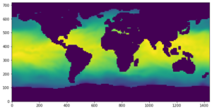
You can get a sense of how the final result looks like by going to HDF Lab and running the example notebook: examples/NEP3/ncep3_example.ipynb (you can see the notebook here as well: https://github.com/HDFGroup/hdflab_examples/blob/master/NCEP3/ncep3_example.ipynb).
While datasets in the original file had the shape (720, 1440), the first dimension representing latitude and the second representing longitude, datasets loaded into HSDS have the shape (7850, 720, 1440). The extra dimension represents time, where the ith element is i days after July 1, 1987.
If we run the hsls command on the aggregated domain we get:
$ hsls -r /home/h5user/NCEP3/ncep3.h5
/ Group
/HDFEOS Group
/HDFEOS/ADDITIONAL Group
/HDFEOS/ADDITIONAL/FILE_ATTRIBUTES Group
/HDFEOS/GRIDS Group
/HDFEOS/GRIDS/NCEP Group
/HDFEOS/GRIDS/NCEP/Data Fields Group
/HDFEOS/GRIDS/NCEP/Data Fields/Psea_level Dataset {7855, 720, 1440}
/HDFEOS/GRIDS/NCEP/Data Fields/Qsat Dataset {7855, 720, 1440}
/HDFEOS/GRIDS/NCEP/Data Fields/SST Dataset {7855, 720, 1440}
/HDFEOS/GRIDS/NCEP/Data Fields/Tair_2m Dataset {7855, 720, 1440}
/HDFEOS INFORMATION Group
/HDFEOS INFORMATION/StructMetadata.0 Dataset {{SCALAR}}
Note that each of the datasets (excepting the scalar dataset) has an extra dimension with an extent of 7855. This domain was created using the hsload --link option, so that actual dataset data is referred to as needed from the original source files. Running hsinfo shows some statistics for the domain:
$ hsinfo /home/h5user/NCEP3/ncep3.h5
domain: /home/h5user/NCEP3/ncep3.h5
     owner: h5user
     id: g-222c9189-6d84ffef-aaa4-1901e5-0c7767
     last modified: 2022-11-30 05:03:14
     last scan: 2022-11-30 05:04:17
     md5 sum: 258a694b2ae0d5c42c39c654bb5d50de
     total_size: 48996941922
     allocated_bytes: 1875928
     metadata_bytes: 18183
     linked_bytes: 48995047555
     num objects: 21
     num chunks: 5
     linked chunks: 31424
You can see the bulk of the data consists of “linked_bytes” which contain 48,995.047,555 bytes (or ~45 GB). These consist of chunk data that resides in the source HDF5 files rather than being copied to the domain. When datasets using linked data are accessed, the service transparently fetches content from the source files as needed.
Accessing the data is a little more straightforward with the aggregated collection. With the original data, in order to construct a time series of all values for a given lat, lon index you would need code like this:
arr = numpy.zeros((7850,), "f4") # construct a numpy array to store retrieved values
for i in range(7850):
     # TBD! - need to convert index to the filename for that day
     filename = get_filename_for_day(i)
     with h5py.File(filename) as f:
          dset = f[h5path] # h5path is path to dataset of interest
          Val = dset[lat, lon] # get data value for lat lon of interest
          arr[i] = val # save to our numpy array
This will be a rather slow process since there’s some overhead with each file open. Also, notice that our TBD function “get_filename_for_day” will be non-trivial to write, or at least an annoyance to deal with.
By contrast, with the aggregated collection the code would look like:
with h5py.File(filename) as f:
     dset = f[h5path]
     arr = dset[:, lat, lon] # retrieve lat/lon value for each day
In this version we have just one file open and one data selection. You can view the complete example in the notebook linked above.
Let’s dive in and explore how you can use hsload to create your own aggregated content in HSDS. There are actually three different methods that can be used. The best approach will depend on how the source files are structured and what you’d like to see for the target datasets. We’ll call these methods “splicing”, “concatenation”, and “extension”. They work as follows:
- Splice: Given that the HDF5 datasets and groups have distinct h5paths, they are combined in the target domain
- Concatenation: Datasets with the same h5path and shape are combined by introducing an extra dimension
- Extension: a specific dimension of datasets with the same h5path is extended
Let’s walk through each of these in turn and how differences should become clear.
If you wish to try these examples out on your own computer, be sure to get the latest h5pyd release: 0.12.1. If you have an earlier release, run: $ pip install h5pyd -upgrade to update.
Splice
Method #1 requires that paths of the source files are all distinct. For example, say you have this collection:
File g1.h5 has dataset: /g1/dsetA
File g2.h5 has dataset: /g2/dsetB
File g3.h5 has dataset: /g3/dsetC
Since none of the object paths conflict, you could combine this to one HSDS domain by running:
$ hsload g1.h5 hdf5://home/myfolder/testone.h5
$ hsload -a g2.h5 hdf5://home/myfolder/testone.h5
$ hsload -a g3.h5 hdf5://home/myfolder/testone.h5
The -a flag in the second two invocations tells hsload not to overwrite the target but to append to it. Since with each hsload none of the objects being added to the domain collide with objects already present, the datasets are created with the same shape, type, and attributes as are in the original files. After the last hsload, testone.h5 will look like this:
/ Group
/g1 Group
/g1/dsetA Dataset {10}
/g2 Group
/g2/dsetB Dataset {10}
/g3 Group
/g3/dsetC Dataset {10}
These commands will copy the data from the source files (so you could delete them afterwards without affecting the HSDS content). If you’d rather not copy the source data but instead link to the source files, you can use the --link option in combination with the -a flag. For example, if the source files are on S3 are:
s3://hdf5_bucket/g1.h5
s3://hdf5_bucket/g2.h5
s3://hdf5_bucket/g3.h5
We’d run:
$ hsload --link s3://hdf5_bucket/g1.h5 /home/myfolder/testone.h5
$ hsload --link -a s3://hdf5_bucket/g2.h5 /home/myfolder/testone.h5
$ hsload --link -a s3://hdf5_bucket/g3.h5 /home/myfolder/testone.h5
When --link is used, rather than the data for each dataset being copied, HSDS just keeps track of where the chunks are located (and which file they are in). Whenever dataset data is needed, HSDS will fetch the required chunk from the source file (so you’ll need to keep the source file around for as long as you’ll be using the HSDS domain).
Note: if you use --link for one file, you’ll need to use it for all files (otherwise the --link -a will fail).
Concatenation
Method # 2 applies if we use hsload -a with objects that will collide with the target. As in the NCEP3 example, in this case an extra dimension will be added for any dataset that is common to the input files.
For example, say are three input files look like this:
HDF5 "file1.h5" {
GROUP "/" {
     GROUP "g1" {
          DATASET "dset" {
               DATATYPE H5T_STD_I32LE
               DATASPACE SIMPLE { ( 10 ) / ( 10 ) }
               DATA {
               (0): 0, 1, 2, 3, 4, 5, 6, 7, 8, 9
               }
          }
     }
}
}
HDF5 "file2.h5" {
GROUP "/" {
     GROUP "g1" {
          DATASET "dset" {
               DATATYPE H5T_STD_I32LE
               DATASPACE SIMPLE { ( 10 ) / ( 10 ) }
               DATA {
               (0): 10, 11, 12, 13, 14, 15, 16, 17, 18, 19
               }
          }
     }
}
}
HDF5 "file3.h5" {
GROUP "/" {
     GROUP "g1" {
          DATASET "dset" {
               DATATYPE H5T_STD_I32LE
               DATASPACE SIMPLE { ( 10 ) / ( 10 ) }
               DATA {
               (0): 20, 21, 22, 23, 24, 25, 26, 27, 28, 29
               }
          }
     }
}
}
Each file has the path “/g1/dset1” where the dataset is a 10-element array. If we aggregate these using the same hsload -a command:
$ hsload file1.h5 hdf5://home/myfolder/testtwo.h5
$ hsload -a file2.h5 hdf5://home/myfolder/testtwo.h5
$ hsload -a file3.h5 hdf5://home/myfolder/testtwo.h5
We get the resultant domain:
$ hsls -r /home/john/aggtest/testtwo.h5
/ Group
/g1 Group
/g1/dset Dataset {3, 10}$
hsls -r /home/john/aggtest/testtwo.h5
/ Group
/g1 Group
/g1/dset Dataset {3, 10}
The three one-dimensional datasets have been concatenated to became one two-dimensional dataset with dimensions: 3 x 10.
If we hsget this domain back to an hdf5 file (so we can run h5dump!), we get:
HDF5 "testtwo.h5" {
GROUP "/" {
     GROUP "g1" {
          DATASET "dset" {
               DATATYPE H5T_STD_I32LE
               DATASPACE SIMPLE { ( 3, 10 ) / ( H5S_UNLIMITED, 10 ) }
               DATA {
               (0,0): 0, 1, 2, 3, 4, 5, 6, 7, 8, 9,
               (1,0): 10, 11, 12, 13, 14, 15, 16, 17, 18, 19,
               (2,0): 20, 21, 22, 23, 24, 25, 26, 27, 28, 29
               }
          }
     }
}
}
You’ll note that the values from the file1 dataset are stored in dset[0,:], values from the file2 dataset in dset[1,:], and values from file3 dataset in dset[3,:].
Like in the first example, you can use the --link option. In this case the resultant dataset will reference data from the three different source files.
The NCEP3 example from the introduction was created using --link and -a from the 7855 HDF5 files in S3. As above, the NCEP3 datasets will have an extra dimension of extent 7855. When you select data with a call such as dset[:, lat, lon], you are in effect reading one element from each of the 7855 S3 objects. Since HSDS can do this in parallel, and has intelligent look up tables to fetch the chunks, you’ll find the operation much faster than opening 7855 files one by one!
Extension
Method #3, works by extending an existing dimension of the combined datasets. Which dimension gets extended is determined by using the extend option in hsload to provide the desired dimension scales. If you are not familiar with dimension scales, this is a useful reference for using them with h5py. Basically, dimension scales are a method of associating one dataset (typically one dimensional) with a specific dimension of a primary dataset. As an example, consider this HDF5 file from the NASA multi-satellite precipitation product:
$ h5ls -r 3B-HHR.MS.MRG.3IMERG.20210901-S000000-E002959.0000.V06B.HDF5
/ Group
/Grid Group
/Grid/HQobservationTime Dataset {1/Inf, 3600, 1800}
/Grid/HQprecipSource Dataset {1/Inf, 3600, 1800}
/Grid/HQprecipitation Dataset {1/Inf, 3600, 1800}
/Grid/IRkalmanFilterWeight Dataset {1/Inf, 3600, 1800}
/Grid/IRprecipitation Dataset {1/Inf, 3600, 1800}
/Grid/lat Dataset {1800}
/Grid/lat_bnds Dataset {1800, 2}
/Grid/latv Dataset {2}
/Grid/lon Dataset {3600}
/Grid/lon_bnds Dataset {3600, 2}
/Grid/lonv Dataset {2}
/Grid/nv Dataset {2}
/Grid/precipitationCal Dataset {1/Inf, 3600, 1800}
/Grid/precipitationQualityIndex Dataset {1/Inf, 3600, 1800}
/Grid/precipitationUncal Dataset {1/Inf, 3600, 1800}
/Grid/probabilityLiquidPrecipitation Dataset {1/Inf, 3600, 1800}
/Grid/randomError Dataset {1/Inf, 3600, 1800}
/Grid/time Dataset {1/Inf}
/Grid/time_bnds Dataset {1/Inf, 2}
In this file, the primary datasets are the ones with dimensions (1, 3600, 1800), e.g. HQobservationTime, IRprecipitation, and precipitationCal, etc. The three dimensions model time, longitude, and latitude. The are also three dimension scale datasets: time, lon, and lat that are attached to the respective dimensions of each of the primary datasets. For example /Grid/lon contains 3600 values specifying the longitude for each index.
This is useful if, say, you are looking at a certain (i,j,k) element in a primary dataset. For this (i,j,k) you can fetch the time, latitude, and longitude by getting time[i], lat[j], and lon[k].
This is useful, but it may seem odd that the time scale only has one element (or that the extent of the time dimension in the primary datasets is just 1). The filename offers a clue.. The substring “.20210901-S000000” in the filename is a hint that this file contains data for September 1, 2021, at midnight GMT (figuring this out requires some trial and error or, in a pinch, by reading the documentation provided for the collection). The next file in the repository is: 3B-HHR.MS.MRG.3IMERG.20210901-S003000-E005959.0030.V06B.HDF5, which indicates it is for time 00:30:00 in the same day.
This suggests an aggregation strategy: combine datasets using the time dimension scale. In this case we are not adding a dimension to the aggregated datasets, but extending the relevant dimension. Since hsload doesn’t know a priori which dimension should be the extended dimension, hsload has an option that can be used to specify this: --extend.
For example, to hsload these two files above, you would run:
$ hsload --extend time 3B-HHR.MS.MRG.3IMERG.20210901-S000000-E002959.0000.V06B.HDF5 hdf5://myfolder/myfile.h5
And then:
$ hsload -a --extend time 3B-HHR.MS.MRG.3IMERG.20210901-S003000-E005959.0030.V06B.HDF5 hdf5://myfolder/myfile.h5
The resulting myfile.h5 will look like:
$ hsls -r hdf5://myfolder/myfile.h5
/ Group
/Grid Group
/Grid/HQobservationTime Dataset {2, 3600, 1800}
/Grid/HQprecipSource Dataset {2, 3600, 1800}
/Grid/HQprecipitation Dataset {2, 3600, 1800}
/Grid/IRkalmanFilterWeight Dataset {2, 3600, 1800}
/Grid/IRprecipitation Dataset {2, 3600, 1800}
/Grid/lat Dataset {1800}
/Grid/lat_bnds Dataset {1800, 2}
/Grid/latv Dataset {2}
/Grid/lon Dataset {3600}
/Grid/lon_bnds Dataset {3600, 2}
/Grid/lonv Dataset {2}
/Grid/nv Dataset {2}
/Grid/precipitationCal Dataset {2, 3600, 1800}
/Grid/precipitationQualityIndex Dataset {2, 3600, 1800}
/Grid/precipitationUncal Dataset {2, 3600, 1800}
/Grid/probabilityLiquidPrecipitation Dataset {2, 3600, 1800}
/Grid/randomError Dataset {2, 3600, 1800}
/Grid/time Dataset {2}
/Grid/time_bnds Dataset {2, 2}
You’ll note that compared to the input files, the aggregated dimension has extent 2, for the time dataset. This dataset contains one value from the first file, and one from the second.
For the primary datasets (e.g. /Grid/precipitationCal), the first extent has been extended from 1 to 2.
You don’t need to stop with two files, as long as you use “--extend time” each new file will expand the time dimensions by 1. On HDFLab you can find an example where a complete day of IMERG data (48 files) is aggregated to hdf5://shared/NASA/IMERG/imerg.2022.09.h5. There’s also a notebook example that walks through accessing the data: https://github.com/HDFGroup/hdflab_examples/blob/master/IMERG/imerg_h5py.ipynb.
One last note: it’s not possible to use the --link and --extend options together.
Conclusion
Hopefully the aggregation options included with hsload will be a useful way to take advantage of the capabilities of HSDS. It can seem a bit confusing at first, but keep in mind that while the aggregation strategy only needs to be figured out once, all users of the resulting collection will benefit. As always, if you have questions on how to use these tools, please post to the HSDS forum or contact help@hdfgroup.org.