David Dotson, doctoral student, Center for Biological Physics, Arizona State University; HDF Guest Blogger
Recently I had the pleasure of meeting Anthony Scopatz for the first time at SciPy 2015, and we talked shop. I was interested in his opinions on MDSynthesis, a Python package our lab has designed to help manage the complexity of raw and derived data sets from molecular dynamics simulations, about which I was
Mohamad Chaarawi, The HDF Group
Second in a series: Parallel HDF5
In my previous blog post, I discussed the need for parallel I/O and a few paradigms for doing parallel I/O from applications. HDF5 is an I/O middleware library that supports (or will support in the near future) most of the I/O paradigms we talked about.
In this blog post I will discuss how to use HDF5 to implement some of the parallel I/O methods and some of the ongoing research to support new I/O paradigms. I will not discuss pros and cons of each method since we discussed those in the previous blog post.
But before getting on with how HDF5 supports parallel I/O, let’s address a question that comes up often, which is,
“Why do I need Parallel HDF5 when the MPI standard already provides an interface for doing I/O?”
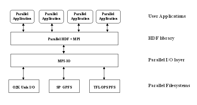
MPI implementations are good about optimizing various access patterns in applications, and the MPI standard supports complex datatypes for scientific data, but that’s how far it goes. MPI does not store any “metadata” for applications, such as the datatypes themselves, dimensionality of an array, names for specific objects, etc. This is where scientific data libraries that build on top of MPI, such as HDF5, come in to help applications since they handle data at a higher level. This diagram describes how parallel HDF5 is layered:
 But now back to our topic.
Parallel I/O methods that HDF5 currently supports: Let’s start with the simple one file-per-process method, where each process creates and accesses a file that no other process is going to access. In this case, the application will program its I/O similar to a serial application, but has to make sure that the file names created between all the processes are not the same. For example, process with rank 0 will access file_0, rank 1 – file_1, and so on… Any VFD can be used in that case to access the files.
The file-per-process is an extreme variation of the more general multiple independent files (MIF) method, where each group of processes accesses independently a single file. The application is programmed such that each process gets a baton giving it a turn to write to the file. When it’s done, it closes the file and passes the baton to the next process in its group. Another extreme variation is to lump all processes in one group making all access done independently to a single file. The overhead of each process opening, closing, and passing the baton could be bad and not scalable on some systems though. The default SEC2 VFD is typically used in that case, but again, any VFD could be used.
So far, all accesses to the HDF5 file(s) are done sequentially by a single process at a time. HDF5 supports parallel access from all processes in a single MPI communicator to a single shared file by using MPI-I/O underneath. To use that, users should set the MPIO VFD to be used by setting the corresponding property in the file access property lists that is passed to the file create or open call:
herr_t H5Pset_fapl_mpio( hid_t fapl_id, MPI_Comm comm, MPI_Info info );The MPI communicator is passed as the comm argument. If all processes will access the file, then MPI_COMM_WORLD is used. The info parameter can be utilized to pass hints to the MPI library. Many of those hints are listed here:
http://www.mcs.anl.gov/research/projects/romio/doc/users-guide.pdf
After creating the file using that FAPL, all processes in the communicator used are now participating in the file access. This means operations that modify the file’s metadata (creating a dataset or writing to an attribute, etc…) are required to be called collectively on all processes. For example, if the user needs to create a 2D 100×200 chunked dataset, with chunk dimensions 10×20, then all processes participating have to call the H5Dcreate() function with the same parameters and the same chunking properties, even if some ranks aren’t actually writing raw data to the dataset. All the operations that have this requirement are listed here: https://support.hdfgroup.org/HDF5/doc/RM/CollectiveCalls.html
Writing and reading raw data in a dataset can be done independently or collectively. The default access mode is independent. Collective access is typically faster since it allows MPI to do more optimization by moving data between ranks for better-aligned file system access. To set collective mode, one needs to set the property on the data transfer property list using the following API call:
herr_t H5Pset_dxpl_mpio( hid_t dxpl_id, H5FD_mpio_xfer_t xfer_mode );and pass the dxpl_id to the H5Dread() or H5Dwrite call. One might ask, “If some processes might have no data to access in a particular raw data access operation, do I need to use independent mode even though most of the processes are participating?” The answer is no. Collective mode can still be used and the processes that aren’t accessing anything will pass a NONE selection to the read or write operation. A NONE selection can be done using:
herr_t H5Sselect_none(hid_t space_id);In some cases, such as when type conversion is required, the HDF5 library “breaks” collective I/O and does independent I/O even when the user asks for collective I/O. This is because the library doesn’t know how to construct the MPI-derived datatypes to do collective I/O. After the I/O operation completes, the user can query the data transfer property list to obtain the I/O method, and the cause of breaking collective I/O if it was broken using the following two API routines respectively:
herr_t H5Pget_mpio_actual_io_mode( hid_t dxpl_id, H5D_mpio_actual_io_mode_t * actual_io_mode);herr_t H5Pget_mpio_no_collective_cause( hid_t dxpl_id, uint32_t
* local_no_collective_cause, uint32_t * global_no_collective_cause);Performance Tuning: Using parallel I/O is one thing, but getting good performance from parallel I/O is another thing. There are many parameters that govern performance and it’s hard to cover them all, but instead I will mention the ones that should always be kept in mind when tuning for performance.
It might be hard to believe, but most queries about bad parallel I/O performance come from the fact that users are using the default parallel file system stripe count (the number of OSTs in LUSTRE). Usually this is set for something very small (like 2). Creating a large file with a large process count with this setting would kill performance. Usually this needs to be adjusted to a better setting. Each HPC system usually has a set of recommended parameters for striping. For example, Hopper @ NERSC has the following recommendations:
http://www.nersc.gov/users/computational-systems/hopper/file-storage-and-i-o
Moving up the stack, we look at MPI-IO parameters. These parameters are usually tunable by info hints. Here are some general parameters that are usually tunable:
- cb_block_size (integer): This hint specifies the block size to be used for collective buffering file access. Target nodes access data in chunks of this size. The chunks are distributed among target nodes in a round-robin (CYCLIC) pattern.
- cb_buffer_size (integer): This hint specifies the total buffer space that can be used for collective buffering on each target node, usually a multiple of cb_block_size.
- cb_nodes (integer): This hint specifies the number of target nodes to be used for collective buffering.
OMPIO, an Open-MPI native MPI-I/O implementation, allows setting those parameters at runtime using OpenMPI’s runtime MCA parameters in addition to setting them through info hints.
Moving further up the stack to HDF5, the current set of tunable parameters includes:
- Chunk size and dimensions: If the application is using chunked dataset storage, performance usually varies depending on the chunk size and how the chunks are aligned with block boundaries of the underlying parallel file system. Extra care must be taken on how the application is accessing the data to be able to set the chunk dimensions.
- Metadata cache: it is usually a good idea to increase the metadata cache size if possible to avoid small writes to the file system. See:
https://support.hdfgroup.org/HDF5/doc/RM/RM_H5P.html#Property-SetMdcConfig - Alignment properties: For MPI IO and other parallel systems, choose an alignment which is a multiple of the disk block size. See:
https://support.hdfgroup.org/HDF5/doc/RM/RM_H5P.html#Property-SetAlignment
Currently however, at the HDF5 level, there are still some issues that cause performance bottlenecks and most have to do with the nature of the small metadata I/O generated by HDF5. The upcoming HDF5 1.10 release should address many of those limitations. (Click here for more information on the upcoming release). A more detailed discussion of those limitations and what we are doing to access them are a subject of a future blog post, so stay tuned on that front!
This FAQ page answers many more common questions about parallel HDF5 usage and performance issues: https://support.hdfgroup.org/hdf5-quest.html#PARALLEL
HDF5 in the Future: The near future of HDF5 should have releases addressing many of the performance bottlenecks that the current 1.8 release has. Also, new API additions are introduced for faster and more convenient file access. But there are still new parallel I/O paradigms that HDF5 doesn’t support.
Current research projects that The HDF Group is leading or involved in include adding support for I/O forwarding capabilities in HDF5. Using an RPC library called Mercury, we can issue HDF5 calls on one machine and have it be executed on another machine. In an HPC system, the source call would be a compute or analysis node, and the destination would be an I/O node or storage server node. Another synergic topic is tiered storage architectures with “Burst Buffers” that are gaining more traction to be the norm for Exascale systems. HDF5 will need to undergo major changes to the data model and file format to fully leverage such systems. Research has been done (and is ongoing with the DOE Exascale FastForward projects) on how to incorporate concepts such as data movements, transactional I/O, indexing, and asynchrony to HDF5.
In summary, there is a lot of work to be done, but the future looks bright for parallel HDF5!presenting a poster (click zip file to download).
In particular, I wanted his thoughts on how we are leveraging HDF5, and whether we could be doing it better. The discussion gave me plenty to think about going forward, but it also put me in contact with some of the other folks involved in the Python ecosystem surrounding HDF5. Long story short, I was asked to share how we were using HDF5 with a guest post on the HDF Group blog.
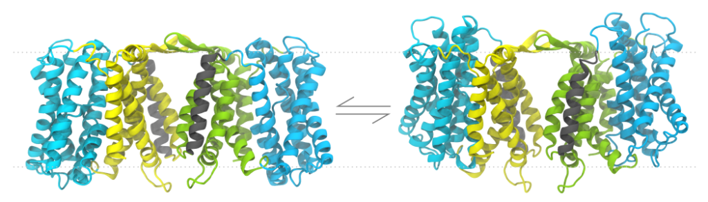
First a bit of background. At the Beckstein Lab we perform physics-based simulations of proteins, the molecular machines of life, in order to get at how they do what they do. These simulations may include thousands to millions of atoms, with the raw data a trajectory of their positions with time, which can have hundreds to millions of frames.
Simulation work often proceeds organically, starting with exploratory simulations with “reasonable” parameters, the results of which inform our next set of simulations and the questions we think we can answer with them. As this process continues, we generate an increasing number and variety of raw trajectories, as well as derived datasets. These datasets can include distances between particular atoms with time, time-averaged spatial densities, radial distribution functions, and anything else we might be interested in. Data from many simulations may be aggregated to build quantitative models, such as Markov state models. Special sets of simulations may also be performed to calculate specific quantities, such as free energies of ligand binding.
We run simulations to examine phenomena that emerge from complexity, but the size, number, and variety of simulations we produce add another layer of complexity that we have a hard time managing. We need to be able to easily sort through the simulations we have, retrieve the datasets we want to explore, and write analysis code that can work across many variants to produce new datasets, ultimately answering biological questions. How can we do this?
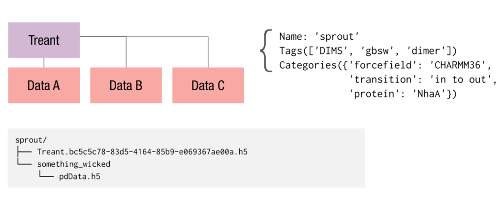
MDSynthesis (MDS) is our answer to this problem, using and abusing HDF5 so we can focus on the science and less on the problem of data storage and curation. MDS gives Treant objects that make storage of pandas objects (Series, DataFrames, Panels) and NumPy arrays as convenient as possible, writing them persistently to disk in individual HDF5 files. Treants live as directory structures in the filesystem, with identifying attributes such as tags and categories (key-value pairs) stored persistently to disk in a state file that is itself HDF5 and managed with PyTables.
For individual simulations, we use a type of Treant called a Sim. These can store additional details such as filepaths for use with MDAnalysis, a domain-specific Python package for picking apart the details of raw MD data. A Sim can also store atom selection definitions, making it easier to write analysis code that works across many simulations even if the details of the selection differ among them.
For aggregating the results of many simulations, we use a Group. This Treant can keep track of other Treants (including any mixture of Sims and Groups) as members, and adds convenience methods for mapping operations on its members in parallel and aggregating their stored datasets.
MDS is a pragmatic tool that is enabled by the flexibility of HDF5, and has greatly improved the speed with which our lab does its work. What’s more, because of its distributed nature (no daemon required, independent objects), it allows us to work with increasingly large datasets without having to set up complex infrastructure. The approach isn’t without its drawbacks, but the advantages are many. It wouldn’t be possible without the versatility and performance of HDF5 and its interfaces in the Python ecosystem, in particular PyTables, h5py, and pandas.
Note: Recently as of this writing, the core components of MDSynthesis have been split off into a package called datreant to be of greater use to domains outside of MD. For any field that works with experimental or simulation data, the package can be used as-is or as a base package for more domain-specific persistent objects. It is still in early development, but already usable. Also, note that there is a lot of historical use of the word “Container” in the docs for MDSynthesis; the word now used is “Treant” to avoid confusion with completely unrelated technologies that are in common use (e.g. Docker).
Editor’s Note:
Thank you so much, David! We loved hearing about your work.
Ideas for guest blogs from others are also welcome – email us at blog@hdfgroup.org.
To see David’s blog, go to http://smallerthings.org/