
by Scot Breitenfeld, Director of Engineering, The HDF Group
For an experiment at the Advanced Photon Source, an aluminum specimen cracked from a corrosion pit to complete failure after 14,346 fatigue cycles. During the process, a micro-CT scanned the specimen, generating 16.8 GB HDF5 files per scan. For this study, we replayed four scans as a live HDF5 stream, processing one checkpoint at a time while an analysis program monitored the crack’s progression. As a result, the program received only 26% of the total data. A live preview accessed just 0.2%, while a traditional streaming method sending every frame to every consumer would have transmitted 500 times more data.
Neither consumer downloaded an entire scan, and the data-writing program required no special modifications. It simply called H5Dwrite(), as any standard HDF5 application would. The key tool is an HDF5 streaming VOL, vol-stream, an HDF5 VOL connector that transforms a regular HDF5 file into a live stream. Readers subscribe to the specific dataset portions they need, and the writer sends only those parts as each step is committed. This post focuses on what this approach looks like in practice.
A crack, 15.7 GiB at a time
The data originates from an in situ fatigue study of corrosion-pitted Al7075, published by Stannard et al. in Corrosion Science 138 (2018), with scans openly available through TomoBank (dataset doi:10.17038/XSD/1373575). Nikhilesh Chawla’s team at Arizona State University soaked peak-aged specimens in 3.5% NaCl before conducting fatigue testing in solution at APS beamline 2-BM-A. Micro-CT scans were performed between cycling rounds. Each scan captured 1,500 projections over 180 degrees using a 2560 × 2160 PCO edge camera at 0.65 µm per pixel and 27.4 keV, along with 10 dark and 10 white frames. All the data was stored as APS DXchange files, resulting in 15.7 GiB of detector data per checkpoint.
The complete series comprises 25 scans, spanning from 750 cycles to final failure at 14,346 cycles, totaling approximately 420 GB. Fourteen scans captured the first 13,000 cycles, while the remaining eleven targeted the final 1,346 cycles, reflecting increased scanning frequency as the crack accelerated. Of these, four scans were chosen for streaming: 750 cycles (specimen intact), 13,000 and 13,800 cycles (crack visible and growing), and 14,346 cycles (after fracture).
Most consumers need a small part of each scan
Every checkpoint captures a full scan, which is an archive requirement. However, few other consumers need the complete dataset. For example, an online analysis node tracking a crack only needs the detector rows intersecting the crack across all projections to reconstruct horizontal slices of that region. In this case, that’s 560 out of 2,160 rows. Meanwhile, a control-room view needs only a single projection to display the current specimen to the operator, plus one dark and one white frame for correction.
Traditionally, you either write the file and let each consumer extract what it needs later or set up a separate streaming path alongside the file. The first approach requires waiting for the file to be complete; the second demands a new data format, additional tools, and another channel to keep in sync. vol-stream offers a third solution: the file itself acts as the stream. Each consumer subscribes to a specific region within the same HDF5 datasets being written, receiving updates for that region as each checkpoint is committed.
The writer just calls H5Dwrite()
Our writer emulates the beamline workflow. For each checkpoint, it opens a step with H5Fbegin_step(), writes the scan’s DXchange datasets (i.e., one projection per H5Dwrite() as the detector provides frames), and finalizes with H5Fend_step(). The fatigue cycle count, not recorded in the scan files, is added as another small dataset alongside the projections. Nothing in this loop knows which clients are listening. The datasets follow the APS layout, maintaining /exchange/data and its dark and white frames, ensuring the file is a valid DXchange file at every checkpoint and can always be reopened later.
The crack monitor is a Python program, and it names its box in the file’s own paths and coordinates:
# rows 400-959 of every projection
f.subscribe({“/exchange/data“: ((0, 400, 0), (1500, 560, 2560))}, expect=shapes)
When the writer calls H5Dwrite() for a projection, vol-stream intersects that write with each subscriber’s designated region and sends only the required data. The monitor receives 560 rows of each projection as a NumPy array matching its specified box. The preview module receives only projection 0; none of the other 1,499 projections are sent to it.
What the crack monitor saw
Each consumer received exactly its designated data at every checkpoint. We ran the writer and both subscribers on a single workstation over TCP. Across four checkpoints, the writer produced a total of 62.6 GiB:
| Consumer | Subscribed box | Received per checkpoint | Share of 15.7 GiB | Deflated in transit |
| Crack monitor | rows 400-959 of every frame | 4.06 GiB | 25.93% | 2.84 GiB |
| Preview | projection 0 + 1 dark + 1 white frame | 31.6 MiB | 0.20% | 20.4 MiB |
At each checkpoint, the monitor determined the rotation center using the first and last projections. It reconstructed eight horizontal slices within its band via filtered back-projection and calculated the proportion of each cross-section that was no longer metal. This process required only NumPy and took 38 seconds per checkpoint. The results matched those obtained by reconstructing the same rows directly from the original scan files, confirming the integrity of the streamed data.
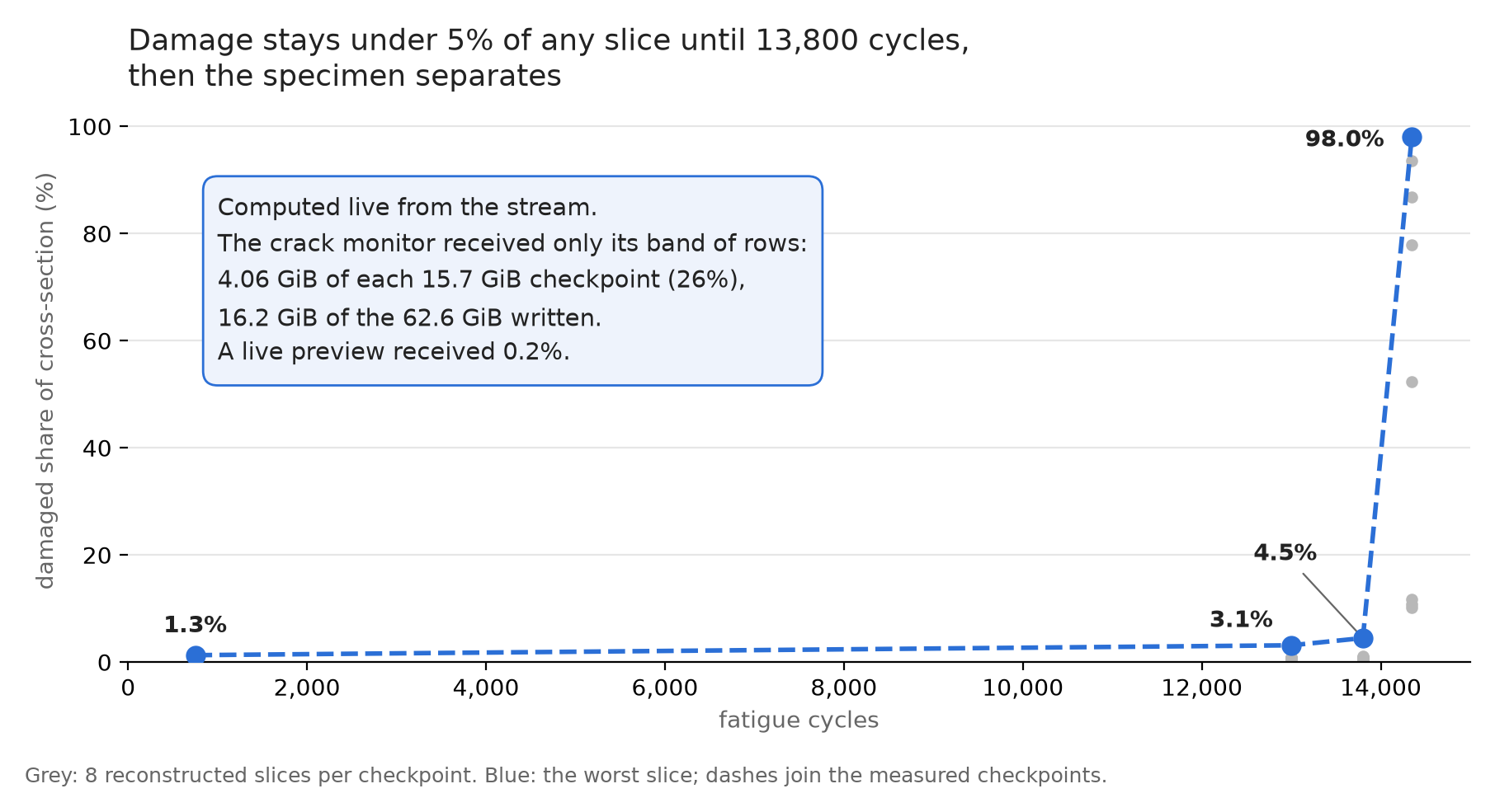
Damaged share of each reconstructed cross-section. Grey: the eight slices per checkpoint. Blue: the worst slice; the dashes join the measured checkpoints.
The crack was first detected as a small fraction of one slice: 3.1% at row 404 after 13,000 cycles, and 4.5% at row 561 after 13,800 cycles. By 14,346 cycles, the lower slices had become almost entirely open gaps, with the most affected reaching 98%. The progression is clear in the slice images: at 750 cycles, the cross-section was a solid alloy with intermetallic particles, surrounded by corrosion products. At 13,800 cycles, a crack propagated inward from the left edge, i.e., the original pit site, leaving open voids nearby. By 14,346 cycles, the slice passed through a gap separating the two halves, now filled with corrosion solution and hydrogen bubbles, corroborating the findings of the original study.
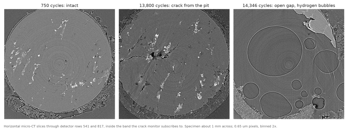
Three micro-CT slices of the same specimen region. Horizontal slices through detector rows 541 and 817, inside the monitor’s band: intact at 750 cycles, a crack running in from the pit at 13,800, and the open gap with hydrogen bubbles at 14,346. The specimen is about 1 mm across.
Sending everything costs 500 times more
Typically, detector data is streamed by sending every full frame to all consumers, leaving each to discard unwanted data. Streams work this way because their basic unit is a frame or message, and it is inefficient whenever a consumer needs only part of each frame. In our experiment, the crack monitor would have received 3.9 times more data and the preview nearly 500 times more. Outgoing traffic from the writer to both consumers would total 31.3 GiB per checkpoint, compared to just 4.09 GiB with directed delivery.
An entire checkpoint takes about 13 seconds to transfer over a 10 Gb/s link and roughly 2 minutes 15 seconds over a 1 Gb/s control-room connection. The preview’s data box transfers in just 0.3 seconds. Over a 25-scan series, sending all data would total about 420 GB per consumer. The crack monitor’s subset would total just 109 GB and the preview only 0.8 GB. The gains extend beyond network savings. The preview never loads a full 15.7 GiB scan into memory just to display one image. Adding an additional consumer only requires the writer to send that consumer’s specific data box, not a full dataset copy.
Subscribers can request in-transit compression, independently of other consumers. Using deflate at level 1 (see the last column in the table above), the writer sent 2.86 GiB instead of 4.09 GiB for the 750-cycle checkpoint. The distribution between consumers is calculated from this total. Compression is lossless, so the monitor’s results remained unchanged. Compression added 46 seconds to the writer’s processing time for that checkpoint. Consumers who do not request compression experience no impact, and the archive file remains unchanged.
The subscription is the point
The key factor here was not faster data transfer, but the ability for each consumer to specify, using the file’s native structure, exactly which part of each checkpoint it required. The writer fulfilled these requests without any change to its own code. The crack monitor, the preview, and the archive all drew from a single stream of standard H5Dwrite() calls, each receiving only relevant data.
The writer, monitor, and orchestration script are available in the vol-stream repository under examples/fatigue_crack. The scan datasets can be accessed via TomoBank’s Globus endpoint. If your instrument outputs HDF5 and multiple consumers require different portions of each frame, define each consumer’s selection and measure actual data transfer before creating a separate pipeline outside the file.
Acknowledgments
vol-stream’s transport layer leverages Mochi components: Mercury handles RPC and RDMA, Argobots provides lightweight threading, Margo integrates these services, and Flock manages group membership. We are grateful to the Mochi development team, especially Matthieu Dorier, for promptly addressing and merging fixes related to Flock issues we reported.
References
- T. J. Stannard, J. J. Williams, S. S. Singh, A. S. Sundaram Singaravelu, X. Xiao and N. Chawla, “3D time-resolved observations of corrosion and corrosion-fatigue crack initiation and growth in peak-aged Al 7075 using synchrotron X-ray tomography,” Corrosion Science 138 (2018). doi:10.1016/j.corsci.2018.04.029
- T. J. Stannard, J. J. Williams, S. S. Singh, A. S. Sundaram Singaravelu, X. Xiao and N. Chawla, “Synchrotron X-ray Tomography for Three-Dimensional Time-Resolved Observations of Fatigue Crack Initiation and Growth from Corrosion Pits in Peak-Aged Al7075 Alloy,” dataset, Advanced Photon Source (2017). doi:10.17038/XSD/1373575
- TomoBank, “In-situ Studies: fatigue-corrosion,” scans tomo_00032 to tomo_00056. tomobank.readthedocs.io
- Mochi documentation. mochi.readthedocs.io
- vol-stream, examples/fatigue_crack: the writer, the crack monitor and the run script used here. github.com/HDFGroup/vol-stream